making_G-R

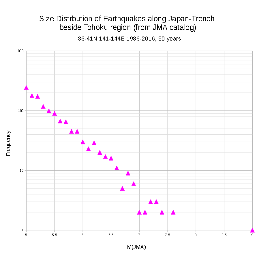
Making Procedure of a size distribution plot of earthquakes from JMA seismicity catalog by Yoshio Okamoto 27th 2019

Data: http://www.data.jma.go.jp/svd/eqev/data/bulletin/hypo.html (It seems to be in Japanese only now.)

1. Combine the data from annual to a period.

cat h1986 h1987 ----- h2015 h2016 > H1986-2016

2. Convert the data format JMA to GMT style

#!/bin/sh
# Data conversion JMA to GMT format
# by Yoshio Okamoto 16/July 2013, 27/February 2019

tr ' ' '_' <H1986-2016> tp1.txt
awk 'substr($0,1,1) == "J"' tp1.txt > tp2.txt
awk '{print substr($0,2,16),substr($0,23,6),substr($0,34,7),substr($0,45,5),substr($0,53,2)}' tp2.txt > tp3.txt
awk 'substr($5,1,1) != "-" && substr($5,1,1) != "_" && substr($5,1,1) != "A" && substr($5,1,1) != "B" && substr($5,1,1) != "C"' tp3.txt > tp4.txt
tr '_' '0' < tp4.txt> tp5.txt
awk '{print substr($0,1,16),substr($2,1,2) "." substr(substr($2,3,4)/6000,3,4),substr($3,1,3) "." substr(substr($3,4,4)/6000,3,4),substr($4,1,5)/100,substr($5,1,2)/10}' tp5.txt > tp55.txt
tr ' ' ',' < tp55.txt> tp6.txt
awk '{print $3" " $2" "$4" "$5 > "JMA1986-2016.dat" }' tp55.txt

rm *.txt

#sort -k 3 -n -r JMA986-2016.dat > JMA1986-2016_ds.dat ## sorting by depth, if it needs.

"JMA1986-2016.dat" is a final one.

3. Pick up the region

#!/bin/sh
# Pick up a area from JMA GMT format data
#　by Y.Okamoto 07/Aug 2013, 27th Feb 2019

# Pick up Area = W/E/S/N or GMT -R
W=141
E=144
S=36
N=41

# picking up by area

awk "{ if ((\$1 >= $W) && (\$1 < $E) && (\$2 >= $S) && (\$2 < $N)) { print \$1,\$2,\$3,\$4 }}" "JMA1986-2016.dat" > Sanriku1986-2016.dat

4. Making Size(M)-Frequency distribution

# count.awk modified 27th Feb 2019 by Yoshio Okamoto
# awk -f JMA_M_count.awk Sanriku1986-2016.dat > Sanriku1986-2016_GR.dat

#main

{
v = $4*10
count[int(v)]++
}

END {
for (v in count) {
print (v/10), count[int(v)]
}
}

5. Use "Excel" or "Calc" to make a scatter plot.

G-R則データ処理備忘録．　2025.11-23

https://earthquake.usgs.gov/earthquakes/search/

よりデータダウンロード．それぞれ2000-2019だと20000の限界を越えるので，いくつかの時間に分けて統合．
されにそれを

grep -v '^time,latitude,longitude' temp.csv > ANSS2000-2019.csv

のように，ヘッダ除去の上，元データとする．これをCGPT作のM_count.shでM別カウント．


DATA_FILE="US_ANSS2000-2019.csv" # ここをあなたのファイル名に置き換えてください

echo "## マグニチュード 0.1 刻みの度数分布表" > G-R2000-2019v2.dat
echo "---" >> G-R.data
echo "マグニチュード_M,度数_n" >> G-R2000-2019v2.data
echo "---" >> G-R.data

# awkで集計し、結果をsortでソートして追記
awk -F',' '
{
    # 5列目 (マグニチュード) がヘッダー "mag" または数値でない場合はスキップ
    if ($5 == "mag" || $5 ~ /[^0-9.]/) {
        next
    }

    # マグニチュードを 0.1 刻みで切り捨て (例: 5.19 -> 5.1)
    M_floor = int($5 * 10) / 10

    # 度数をカウント
    M_COUNT[M_floor]++
}

END {
    # ソートされていない順で出力し、外部の sort コマンドに任せる
    for (M in M_COUNT) {
        print M "," M_COUNT[M]
    }
}' "$DATA_FILE" | sort -n -t',' -k1,1 >> G-R2000-2019v2.dat


これでOK．

SEAsia，Japan, USを作成．

それぞれ，範囲は85-130，0-30
125-150，25-50
-130　-100，25-45

さらに，この地図範囲を描画するHTMLをCGPTで作成．



<!doctype html>
<html lang="ja">
<head>
  <meta charset="utf-8" />
  <title>世界地図に矩形を描く（Leaflet） - 複数矩形対応</title>
  <meta name="viewport" content="width=device-width, initial-scale=1.0">
  <link rel="stylesheet" href="https://cdnjs.cloudflare.com/ajax/libs/leaflet/1.9.4/leaflet.css">
  <style>
    html,body,#map { height: 100%; margin: 0; padding: 0; }
    .controls { position: absolute; top: 8px; left: 8px; z-index: 1000; background: rgba(255,255,255,0.95); padding:8px; border-radius:6px; font-size:13px; box-shadow: 0 1px 6px rgba(0,0,0,0.2)}
    .controls input { width: 110px }
    .controls .row { margin-bottom:6px }
    .legend { position: absolute; bottom: 8px; left: 8px; z-index:1000; background: rgba(255,255,255,0.9); padding:6px; border-radius:6px; font-size:12px }
    .btn { padding:6px 8px; margin-left:6px }
  </style>
</head>
<body>
  <div id="map"></div>
  <div class="controls">
    <div class="row">北 (N): <input id="inpN" value="45"></div>
    <div class="row">南 (S): <input id="inpS" value="10"></div>
    <div class="row">西 (W): <input id="inpW" value="120"></div>
    <div class="row">東 (E): <input id="inpE" value="150"></div>
    <div style="margin-top:6px;text-align:right">
      <button id="drawBtn">描画</button>
      <button id="clearBtn" class="btn">全削除</button>
      <button id="toggleMarkers" class="btn">マーカー表示: ON</button>
    </div>
    <div style="margin-top:6px;font-size:11px;color:#333">座標は度（十進）で入力してください。西経/南緯は負の値。複数矩形は色が順に変わります。</div>
  </div>
  <div class="legend" id="legend">矩形数: 0</div>

  <script src="https://cdnjs.cloudflare.com/ajax/libs/leaflet/1.9.4/leaflet.js"></script>
  <script>
    const map = L.map('map').setView([30, 135], 3);
    L.tileLayer('https://{s}.tile.openstreetmap.org/{z}/{x}/{y}.png', { maxZoom: 19, attribution: '&copy; OpenStreetMap contributors' }).addTo(map);

    const colors = ['#ff0000','#0000ff','#00aa00','#ffaa00','#aa00ff','#00cccc','#ff66cc','#6666ff'];
    let colorIndex = 0;
    const rectLayers = []; // {layer: L.rectangle, corners: [markers...]}
    let showMarkers = true;

    const legend = document.getElementById('legend');
    function updateLegend(){ legend.textContent = '矩形数: ' + rectLayers.length; }

    function normalizeLon(lon){ // -180..180
      let x = Number(lon);
      if (x > 180) x -= 360;
      if (x < -180) x += 360;
      return x;
    }

    function addRectangle(N,S,W,E){
      const north = Number(N); const south = Number(S);
      const west = normalizeLon(W); const east = normalizeLon(E);
      const bounds = [[south, west],[north, east]];
      const color = colors[colorIndex % colors.length];
      colorIndex++;

      const rect = L.rectangle(bounds, {color: color, weight: 2, fillOpacity: 0}).addTo(map);
      const markers = [];
      if (showMarkers){
        const NW = [north, west];
        const NE = [north, east];
        const SE = [south, east];
        const SW = [south, west];
        const names = ['NW','NE','SE','SW'];
        [NW,NE,SE,SW].forEach((c,i)=>{
          const m = L.circleMarker(c,{radius:4, fill:true}).addTo(map).bindPopup(names[i] + ': ' + c[0].toFixed(6) + ', ' + c[1].toFixed(6));
          markers.push(m);
        });
      }

      rectLayers.push({layer: rect, markers: markers});
      fitAllBounds();
      updateLegend();
    }

    function fitAllBounds(){
      if (rectLayers.length === 0) return;
      let group = L.featureGroup(rectLayers.map(r=>r.layer));
      map.fitBounds(group.getBounds().pad(0.2));
    }

    function clearAll(){
      rectLayers.forEach(r=>{
        map.removeLayer(r.layer);
        r.markers.forEach(m=>map.removeLayer(m));
      });
      rectLayers.length = 0;
      updateLegend();
    }

    document.getElementById('drawBtn').addEventListener('click', ()=>{
      const N = parseFloat(document.getElementById('inpN').value);
      const S = parseFloat(document.getElementById('inpS').value);
      const W = parseFloat(document.getElementById('inpW').value);
      const E = parseFloat(document.getElementById('inpE').value);
      if (isNaN(N)||isNaN(S)||isNaN(W)||isNaN(E)) { alert('数値で入力してください'); return; }
      if (S >= N) { alert('南(S) は 北(N) より小さくしてください'); return; }
      if (Math.abs(E - W) > 360) { alert('経度差が不正です'); return; }
      addRectangle(N,S,W,E);
    });

    document.getElementById('clearBtn').addEventListener('click', ()=>{ clearAll(); });

    document.getElementById('toggleMarkers').addEventListener('click', (ev)=>{
      showMarkers = !showMarkers;
      ev.target.textContent = 'マーカー表示: ' + (showMarkers? 'ON':'OFF');
      // 既存マーカーを表示/非表示
      if (showMarkers){
        rectLayers.forEach(r=>{
          // create markers again from rectangle bounds
          const b = r.layer.getBounds();
          const north = b.getNorth(); const south = b.getSouth();
          const west = b.getWest(); const east = b.getEast();
          const NW = [north, west]; const NE = [north, east]; const SE = [south, east]; const SW = [south, west];
          const names = ['NW','NE','SE','SW'];
          const newMarkers = [];
          [NW,NE,SE,SW].forEach((c,i)=>{
            const m = L.circleMarker(c,{radius:4, fill:true}).addTo(map).bindPopup(names[i] + ': ' + c[0].toFixed(6) + ', ' + c[1].toFixed(6));
            newMarkers.push(m);
          });
          r.markers = newMarkers;
        });
      } else {
        rectLayers.forEach(r=>{ r.markers.forEach(m=>map.removeLayer(m)); r.markers = []; });
      }
    });

    // 最初の描画
    addRectangle(45,10,120,150);
  </script>
</body>
</html>

G-R則用のデータセット作成　備忘録　　7thApr．２０１２

ANSSから１９９２年ー２０１１年で30-40N，95-85Wでデータを抽出．これをNMSZ.datとする．
ここから，諸元を抜いた数字だけのデータをNMSZ.txtとする．
度数分布作成カウントは
http://macroscope.world.coocan.jp/ja/edu/computer/awk/griddata/main.html
より，

# count.awk

#main

{
v = $6*10
count[v]++
}

END {
for (v in count) {
print v/10, count[v]
}
}

を作成．実行パーミッションを付けて，
awk -f ANSS_count.awk NMSZ.txt>out.txt
でOK．
out.txtは

1 97
1.1 101
1.2 150
2 303
1.3 205
2.1 276
1.4 282
2.2 266
1.5 506
3 30
2.3 219
1.6 509
3.1 32
2.4 173
1.7 403
3.2 19
2.5 187
1.8 334
という感じ．これをGMTでグラフ化することを考える．
と思ったが，とりあえずエクセルに読ませてグラフ化するほうが簡単．

あと，理科年表の気象庁のデータを手入力して同様の処理．